Introduction

GAC and the Aquarium

The use of granular activated carbon (GAC) for decolorizing marine aquarium water has had a long and successful history. In fact, prior to the introduction of this filtering agent into the saltwater aquarium hobby, the central role of this technology in water remediation efforts ensured that a large body of data existed which spoke to the basics of contaminant removal from drinking water and wastewater by carbon-based media (Bansal, 2005; Cheremisinoff, 1993; Kvech, 1997). Through extensive experimental and theoretical (i.e., model building) studies, many of the parameters that define success have been identified. Optimization of GAC source, water flow rate through fixed-bed reactors, media presentation, and time-in-use, among other features, has led to successful protocols for the removal of many small-molecule organic contaminants, such as benzene, phenol, chlorinated hydrocarbons, pesticides, etc. from potable water sources (Bansal, 2005; Khan, 1997; Singh, 2006). It is not surprising that many of the lessons learned from these studies accompanied the technology as it was adapted to marine aquarium use. Some empirical and largely divergent “rules for use”, which have emerged from these initial inputs combined with the numerous observations of aquarists, have been proposed by many authors (http://www.carbochem.com/activatedcarbon101.html; http://www.articlefishtalk.com/Article/Activated-Carbon-in-the-Aquarium/78; Hovanec, 1993; Harker, 1998; Schiemer, 1997). Although there is by no means a uniform consensus, recommendations 1 and 2 below seem to have stood the test of time. On the other hand, opinions conflict on the questions of how much (#3), how fast (#4), and how often (#5).

1. Use GAC formulated from either bituminous coal (Hovanec, 1993) or lignite coal (Harker, 1998), but not coconut shell.
2. Use active flow through the media and not passive diffusion (Hovanec, 1993; Harker, 1998).
3. Use about 0.3 gm of GAC per gallon of tank water (“3 tablespoons per 50 gallons”) (Harker, 1998) to 19 gm/gal (Lliopoulos, 2002) (no consensus here).
4. Use water flow rates of about 4 gph (Harker, 1998) to several hundred gph [many canister filter manufacturers] (again, no consensus).
5. Replace with new GAC every week (Harker, 1998) to once every 4-6 weeks (Schiemer, 1997) (once again, no consensus).
6. Run continuously (Schiemer, 1997) or sporadically (Harker, 1998) (no consensus!).

Dissolved Organic Carbon

The precise chemical species that GAC removes have not been determined. Rather, the catchall phrases “DOC” (dissolved organic carbon) and/or “marine humic/fulvic acids” are frequently employed to categorize the uncharacterizable (Holmes-Farley, 2004; Bingman, 1996; Rashid, 1985; Romankevich, 1984). In fact, both descriptors have little intrinsic meaning and give no insight into the actual chemicals involved. Romankevich has estimated that there is approximately 2 x 10¹² tons of DOC in the world’s oceans (for comparison, Romankevich reports that there are approximately 2.5 x 10¹² tons of organic carbon in oil deposits in the world), and about 94% of that material is phytoplantonic in origin (Romankevich, 1984). Most (all?) of these dissolved organic materials are subjected to both biological (bacterial) and non-biological degradative processes until eventually refractory (= inert) compounds, which survive exposure to the marine environment’s inhabitants and conditions, result. Occasionally, marine scientists have attempted to provide some structural details for these substances on the basis of the spectroscopic signatures of specific chemical functionalities observed. In particular, solid-state carbon nuclear magnetic resonance spectroscopy has provided an unrivaled window into this complex problem (Gillam, 1986; Sardessal, 1998). Representative polycyclic species derived from oxidation and then cyclization of unsaturated lipids have been proposed (Harvey, 1983), whereas other authors have suggested that some humic acid components originate from oligosaccharide-protein condensations to form polycyclic materials that have a high nitrogen content (Francois, 1990). The former process has a direct analogy to the curing of oil-based varnishes for wood treatment, whereas the latter process is related to the chemistry of food browning upon cooking, a sequence of transformations called the Maillard reaction. In both cases, colored, soluble material can be formed. Both of these chemical transformations require condensation of different chemical reaction partners that each exist in concentrations of approximately 1 ppm, and so any hypothesis for DOC formation that cites these reactions must address this low-concentration-of-reactants issue.

Our Experimental Goals

With this information as background, we set out to experimentally probe some of the unresolved issues surrounding the use of GAC in the marine aquarium:

1. How much GAC should be used to deplete the DOC by 90% (arbitrarily chosen) for a given water volume?
2. When should the GAC charge be changed?
3. Does GAC differentially remove different types of arguably reef-relevant organic molecules with different facility? That is, are all yellow, or more generally, colored, compounds removed with equal facility, and are there non-yellow-colored but possibly undesirable organic compounds that GAC removes as well?
4. How does the rate of impurity removal relate to water flow rate?
5. Do organics leach back out of GAC upon saturation?

Some tentative answers (not THE answers) to these questions are presented below.

Prior to framing these questions in experimentally addressable terms, some basics must be considered: For example, what experimental quantity should be measured – the amount of the impurity that a given amount of GAC removes, or the rate by which the GAC removes the impurity? Actually, both quantities will be required to address these questions. Historically, measurements of the ability of GAC to remove an impurity from water have looked at both issues. Some background:

1. Thermodynamics. Thermodynamic measurements attempt to describe the quantity of impurity that can be removed by a given quantity of GAC (Suzuki, 2004; Walker, 2000). These types of measurements are run to “infinite” time; that is, the system (= GAC + impurity in water) is allowed to settle until the measured concentration of impurity in the water is constant; or, in chemical terms, the system has reached equilibrium. From these measurements of GAC’s adsorbing capacity (different for each chemically unique impurity) and application of mathematical treatments relying on either the Freundlich or Langmuir isotherms [Potgieter, 1991], many useful system parameters can be calculated. This type of analysis provides data pertaining to which type of GAC can adsorb the most impurity-per unit-weight. Many authors have applied this technique in analyzing the use of GAC with marine aquaria, and some of their conclusions (cf. # 1 and # 5 in the Introductory section) have been presented. These data do not address how fast impurities are removed.
2. Kinetics. Kinetic measurements attempt to describe how fast GAC removes an impurity (Ganguly, 1996; Baup, 2000). These data do not reveal the ultimate adsorption capacity of the GAC. The kinetic approach to developing figures of merit for GAC has been explored by some aquarist authors (Cerreta, 2006; Walker, 1999; Harker, 1998), and conclusions about active vs. passive flow (# 2 above), preferred type of GAC precursor (#1 above), and amount of GAC to use (# 3 above) have been derived from these data.

It should be emphasized that the kinetic approach and the thermodynamic approach actually measure different things, and data garnered from these two different experimental protocols will not necessarily lead to the same conclusions about which is the “best” GAC, depending upon the criteria used to define “best”. It is possible, for example, for a particular sample of GAC to remove an impurity very rapidly but actually have a rather low capacity. Conversely, another sample of GAC may exhibit the exact opposite behavior; there is no reason why the kinetics of impurity removal and the capacity of the GAC sample should correlate or even run in parallel.

These assertions can be better understood when viewing GAC on the molecular level. As many authors have detailed in earlier accounts (Hovanec, 1993; Kvech, 1997), GAC is essentially a refractory solid honeycombed with passages and chambers that are chemically active enough to bind some types of organic molecules. The sizes of the interior spaces are exceedingly heterogeneously distributed, and vary as per the technique(s) used to activate the carbon. Likewise, the chemical nature of the active binding surfaces is heterogeneous and the details of the surface molecular constituents depend upon the activation procedure. This heterogeneity all works towards the good, as GAC in the aggregate then offers many differently sized and functionally distinct binding sites to act as complementary partners for the myriad of structurally different organic impurities that might be found in a marine aquarium, lumped under the aegis of DOC. The thermodynamics (= capacity at equilibrium) of impurity removal typically scales with the number, or amount, of available binding sites for impurities. If a GAC sample has a greater porosity due to its activation procedure, it will have the capacity to trap and hold more impurity. The kinetics (= rate of impurity capture) of DOC removal is dependent on several factors: (a) the rate of diffusion of the impurity to the surface of the GAC particle, (b) the rate of diffusion of the impurity inside the potentially restricting space of the pores, (c) the rate of surface diffusion once the impurity is bound, and (d) the strength of the specific molecular-level interactions between the GAC surface and the impurity in question. All of these rate components are sensitive to the specific shape, charge, size and chemical functionality of the impurity. Therefore, there is no real correlation, or expectation of a correlation, between the amount of surface area for binding within the pores and channels in GAC (proportional to thermodynamic capacity) and the diffusion rates and surface chemistry within these pores and channels (influences the kinetic rate of removal).

Both kinetic and thermodynamic data are necessary for probing the central questions outlined above. Quantifying the rates of impurity removal (kinetics) as a function of different chemical impurity structures will allow question (3) to be tested, whereas the kinetic approach will directly address the questions posed in (1) and (4). Measurement of impurity leaching rates of impurity-saturated GAC (question (5)) will address concerns that used GAC itself might be a source of DOCs if not removed when saturated. Finally, the GAC’s thermodynamic adsorption capacity should provide direction with question (2).

The Mathematical Models

There are two distinct tank scenarios that require different mathematical models to obtain useful information.

1. There is a fixed amount of impurity (DOC), and no more is being added, at least at a rate competitive with the rate of impurity removal by the GAC. This case most likely might be encountered if GAC has not been used for a while, and so the DOC level has built up, or if the tank has been medicated, and it is important to remove excess medication quickly. The key question here is, “How much GAC should I use to remove this large amount of impurity?”
2. GAC is in continuous use, and the steady-state DOC level reflects the trade-off between the rate of DOC introduction by biological processes, and the rate of DOC removal by the GAC. This situation would pertain if GAC is used continuously. The key question here is, “When should I change my GAC?”

We will first examine scenario (1), and then use the results obtained to arrive at an approach to address scenario (2).

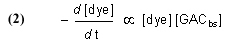
The fundamental Case 1 chemical equation that describes the removal of an organic dye molecule (as a model for DOC) from solution by GAC is

Note that this equation does not have any provision for adding dye to the water, and so it describes Case (1) and not Case (2). The symbol “GAC_bs” in this chemical equation is defined for our purposes as one binding site in the GAC matrix. In words, this equation indicates that one molecule of dye (or one mole, which equals 6.02 x 10²³ molecules – it is often convenient to discuss chemical process in terms of moles, or fractions of a mole – millimol, micromol, etc.) binds to one binding site in the GAC (or one mole of binding sites) and therefore is removed from solution. An assumption of this model is that the dye can leach from the GAC and reenter the solution, leading to a situation called “equilibrium binding”. That is, the GAC will become saturated with dye at some point, and that saturation point is a complex function of how much dye is present, how much GAC is present, and the molecular-level affinity of the GAC for the dye. A test of this assumption will be described later in the article. This one-to-one interaction between the dye molecule and a GAC binding site (GAC_bs) lends itself to a mathematical analysis characterized by the relationship in Eq. (2). In words, this expressions indicates that the rate of removal of dye from solution (symbolized by the differential –d[dye]/dt, t = time in minutes) is proportional to the product of the concentration of dye (in moles per liter, often abbreviated as mol/L, or M, and indicated by the symbol [dye]), and the concentration of GAC binding sites available ([GAC_bs], in moles per liter of total solution). Of course, the GAC binding sites are not spread throughout the whole solution, but rather they are confined to the GAC particles in a Phosban (or equivalent) reactor. However, the experimental design is such that this distinction is not significant. This proportionality expression can be converted to an equality by including a constant of proportionality denoted as k (Eq. (3)).

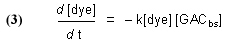
Although it may seem that the introduction of this “fudge factor” k is somewhat arbitrary and perhaps not even germane to the problem, it turns out that it is possible to use this single figure-of-merit to describe the key rate characteristics of the system – k is often called a rate constant. The larger k is, the faster that the GAC removes the dye from solution. Note that k is independent of the amount of GAC used – in principle, the same k should be obtained for any amount of GAC from the same source. In practice, we shall see that the reality is somewhat different, perhaps reflecting the crudeness of some of the assumptions of our model, and the inconsistencies that attend any repetitive experimental measurement procedure. Whereas the rate constant k should be invariant with respect to GAC amount, the actual rate of dye removal (d[dye]/dt) is a function of the amount of GAC present, since the amount of GAC binding sites ([GAC_bs]) will scale with the amount of GAC used. In typical aquarium use, the amount of DOC will be relatively small and constant, and the amount of GAC used is the real variable available to the aquarist in terms of accelerating the removal of unwanted DOC’s.

It will be our goal to calculate this value k under different conditions. The rate constant k is a function of all of the intrinsic features of the system, such as the flow rate through a Phosban Reactor, the physical configuration of the plumbing and Reactor, the dimensions and aspect ratio of the GAC bed, the GAC particle size and porosity, the diffusion rate to the GAC surface and along the GAC surface/pores as discussed earlier, etc. It is not possible at this level of analysis to deconvolute the calculated k value in terms of these specific parameters, but it is possible to use this rate constant value for a given set of experimental parameters to calculate useful attributes of the system, such as (1) how long will it take to cut the amount of dye (or DOC) by 90% for a given tank size and GAC amount, and (2) how long will it take to saturate 90% the GAC binding sites with dye (or DOC’s in a real aquarium) for a given tank size and GAC amount. These practical issues will aid in making informed decisions on the related questions of “How much GAC should I use?” and “When do I need to change my GAC?”

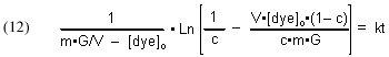
It is possible to derive a mathematical expression from Eq. (3) that relates the desired rate constant k to experimentally measurable (or derivable) quantities. This derivation can be found in any standard Chemical Kinetics treatment/textbook, and the expression is

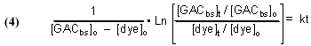
where

t = time, in minutes

[dye]_t = the concentration of dye, in moles/liter (M), at time t

[dye]_o = the concentration of dye (M) at t = 0 (i.e., the beginning of the experiment)

[GAC_bs]_t = the concentration of binding sites in the GAC, in moles/liter (M) at time = t

[GAC_bs]_o = the concentration of binding sites in the GAC (M) at t = 0

k = rate constant from Eq. (3), in M^-1min^-1

We can measure [dye]_o, the amount of dye that we put into the system in the beginning, and we can measure [dye]_t, the concentration of dye at some time t after the experiment begins. Obtaining the other necessary quantities, [GAC_bs]_o and [GAC_bs]_t, requires some mathematical manipulation and some assumptions.

The total binding capacity of the GAC, which is equal to [GAC_bs]_o, can be indirectly measured by placing a known quantity of GAC in solution with a known and excess quantity of dye. The GAC will absorb the dye until it becomes saturated and can no longer bind any more dye. As a consequence, the concentration of the dye in solution will decrease as some of the dye is bound to the GAC. Eventually, the concentration of dye in solution will remain constant, as the now saturated GAC can no longer accept any more dye. We can monitor the decrease in dye concentration over time, and when the concentration levels out and no longer changes, we assume that we have reached the GAC saturation point. The difference in dye concentration between the initial value and this terminal value can be used to determine the amount of dye absorbed by the GAC, and we can use a mathematical treatment called a Langmuir isotherm to calculate the total binding capacity of the GAC for the dye. The mathematical form of the Langmuir isotherm is given in Eq. (5) [Potgieter, 1991]:

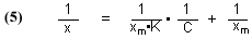
where

x = milligrams (mg) of dye absorbed per mg of GAC, at equilibrium

C = the concentration of dye (mg/L), at equilibrium

K = a constant of no interest in this analysis

x_m = the total amount of dye (mg) that can be absorbed by 1 mg of GAC, at equilibrium

The total binding capacity of the dye is x_m, the quantity that we seek. Simply running several parallel trials to equilibrium, all differing in the amount of GAC used (leading to differing x values), and measuring the dye concentration, C, will provide the necessary data. Then, plotting 1/C vs. 1/x should provide a straight line whose Y-intercept is 1/x_m. The desired quantity for this experiment, x_m, is then in hand.

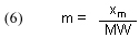
In order to use this experimentally derived quantity of binding capacity, x_m, to calculate [GAC_bs]_o, we must define a new quantity, m, as the # of moles of dye that bind to one gram (abbreviated 1g) of GAC at equilibrium. Note that x_m originally is determined in units of mg of dye/mg of GAC, but that ratio is equivalent to gms of dye/gms of GAC. Thus, simply dividing x_m by the dye’s molecular weight (MW, in g/mol) provides m:

In addition, [GAC_bs]_o requires knowledge of the system water volume (V) and the amount (mass) of GAC used (G):

V = the volume of the water in the system, in liters (experimentally measured)

G = the grams of GAC used (experimentally measured)

So, m•G = the total # of moles of binding sites for a given mass of GAC, and therefore

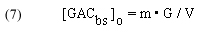
In words, this expression indicates that the concentration of the total amount of GAC binding sites is equal to the total # of moles of binding sites divided by the system volume. As indicated earlier, the GAC binding sites are not evenly dispersed throughout the solution, but are confined to the GAC bed. This distinction is of no consequence, however, since our experimental protocol is equivalent to just adding a portion of GAC to the tank volume itself. The fact that dye can only be removed when the solution passes through the GAC bed is taken into account by the rate constant k.

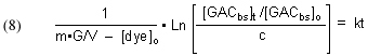
In addition, it is convenient to formulate another definition:

c = [dye]_t/[dye]_o, which again is an experimentally measured quantity.

Substituting these two expressions into Eq. (4) leads to

Arriving at a experimentally accessible expression for [GAC_bs]_t is a bit trickier. We can start by noting that there is a fundamental mass balance expression that defines the removal of dye by GAC:

In words, this expression indicates that the amount of dye removed from solution up to a time t (= [dye]_o – [dye]_t) must be equal to the amount of dye absorbed onto the GAC during that same time, which, in turn, must equal the decrease in the amount of GAC binding sites (= [GAC_bs]_o – [GAC_bs]_t). Rearranging and substituting for [dye]_t gives

Substituting back into Eq. (8) then gives

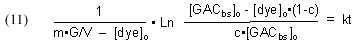
Substituting [GAC_bs]_o = m•G/V and rearranging furnishes

which simplifies to

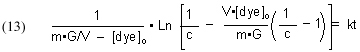
The quantities m (derived from the Langmuir isotherm experimental data) and [dye]_o are measured initially, and remain constant throughout all of the experiments. The amount of GAC, G, is measured at the beginning of each experimental run, and [dye]_t (from which c is derived) is measured at different times t. The quantity on the left-hand side of Eq. (13) is graphed against time t, and the slope of that line is k, the desired quantity.

It will be valuable to define a new quantity, t₉₀, as the length of time required to reduce a given starting dye concentration by 90%. The t₉₀ value can be extracted from Eq, (13) by setting c = 0.1 (= 90% depletion of the dye concentration), and solving for t:

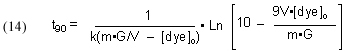
This Case (1) mathematical modeling ultimately can be applied to answering the question, “How much GAC should I use?” (see Section 3.1). That is, this model will have the most utility is a situation where GAC has not been used before, and the DOC level in the water has built up, or a situation where the tank has been medicated, and so there is a specific level of impurity (excess medication) that must be removed quickly.

To address the Case (2) scenario, where GAC is used continuously and DOC (modeled by dye) is continuously being added to the water, we must explicitly incorporate a DOC source into the simple expression Eq. (1). Specifically, we can allocate that role to PoOP (Precursors of Organic Particulates), and then assign a generic rate constant k₁ to describe the overall rate of conversion of PoOP into DOC’s (modeled by dye in Eq. (15)). This simplistic model allows for a continuous and gradual introduction of DOC’s (dyes) into the water column of an aquarium as a consequence of a wide range of biological processes that degrade the PoOP into soluble organic material. Thus, Eq. (15) illustrates how dye (as a model for DOC) is both formed from PoOP with a rate constant k₁, and removed by the GAC with a rate constant k, as previously discussed.

Surprisingly, the expansion of Eq. (1) into Eq. (15), which includes the dye generation term, renders the kinetics mathematically unsolvable, at least in terms of arriving at an analytical solution like that expressed in Eq. (13). This problem has long been recognized, and Chien has developed a workaround using mathematical approximations (Bessel functions) that are applicable if certain criteria are met (Chien, 1948). However, there are two factors that mitigate against using the Chien formalism to solve this problem:

1. It is not clear whether the criterion for its use, which involves the relative magnitudes of k and k₁, is met.
2. We can only guess at the concentration of PoOP and the value of the rate constant k₁ (necessary inputs for Chien’s mathematical model).

This second point is really a critical one, as it will cloud any attempt to arrive at a solution based on Eq. (15). However, all is not lost, as there is another approach to solving kinetic (rate) expressions that is applicable in this case; kinetics simulations. It is possible to use one of the commercially available kinetics modeling programs to make guesses for [PoOP] and k₁, and then calculate desirable quantities like [GAC_bs]_t or [dye]_t based on experimentally determined k values (from the Case (1) math and experimental measurements). Even with this approach, we must have some basis for making guesses about [PoOP] and k₁, and fortunately, we do. As discussed later in more detail, we have measured the concentration of oxidizable organics in the water of several reef tanks, and so we have an idea of the steady-state concentration, [DOC], in an actual GAC-treated tank. With that constraint, we can then adjust the product [PoOP]•k₁ in the kinetics simulation program to hold [DOC] within a realistic range. That is, the rate of DOC removal will be measured experimentally, and then we just have to balance that rate of removal with a rate of DOC introduction via a [PoOP]•k₁ quantity that keeps the overall DOC level around the steady-state values measured in actual marine tanks. For these studies, we use the shareware program KinTekSim (http://www.kintek-corp.com/members/).

The Experimental Variables

The experimental variables examined in this study are:

1. The type of GAC: Two Little Fishes Hydrocarbon and Marineland’s Black Diamond.
2. The flow rate: 49 gph (= 0.81 gpm) and 72 gph (= 1.2 gpm).
3. The amount of GAC: 6.25 g/gal up to 50 g/gal.
4. The dye molecule probes. This latter experimental variable is quite important to the success of these experiments, and so some more elaboration and a few digressions are in order. First, a digression about the pros and cons of model use in science:

Some scientific disciplines have a “look but don’t touch character” to their experimentation. For example, cosmology and paleontology ask questions about events so distant in time (the birth of the Universe or the behavior of dinosaurs) that it is impossible to construct real-time experiments to gain hard data. Thus, model building and model testing are the primary experimental tools of these types of disciplines. Other fields of science are readily probed by direct experiment, like chemistry and biology. However, even within these hands-on sciences, the type of experiments, and the quality of data retrievable, varies significantly. For example, directly probing a biological or chemical system of interest is possible, but sometimes the system is so complicated that the data obtained is uninterpretable or compromised. For example, such a situation might pertain to the question of what, exactly, is GAC removing. Sure, it can be labeled as “DOC”, or “marine humic substances”, but those categories reveal nothing about its chemical structure and hence its reactivity with GAC or any other component of an aquarium. In reality, the DOC is so complex and so heterogeneous that it would be a Herculean analytical task to try to determine its constituents and their relative amounts. So, how can experiments whose goal involves DOC chemistry be performed? In principle, it might be possible to isolate and concentrate DOC, and use that preparation as an experimental starting point without ever knowing its composition. That type of procedure would hew closest to the goal of performing experiments on a “real” system, but the downsides of this approach are many: there is currently no effective way to isolate all of the DOC’s, although some subset of DOC components can be isolated; there is no effective way to ensure that whatever might be isolable actually corresponds to the DOC of an aquarium; there is no way of testing whether the DOC isolated from one aquarium is similar to, or different from, the DOC isolated from another aquarium. In light of these types of technical (but not conceptual!) problems in working with complex “real” systems, scientists often turn to simplified model systems that presume to capture the essential elements of the real system but reduce the experimental variables to a manageable number. In this approach, experiments can be designed and executed, but the real challenge lies in choosing appropriate model systems that can give insight into the real system. In the case of GAC and DOC removal studies, several authors used a blue dye, the Salifert test kit reagent methylene blue (1), as a model for organic impurities that might be found in a reef tank (Cerreta, 2006; Schiemer, 1997). Harker, on the other hand, used the yellow exudates from stewed seaweed as a model for DOC, reasoning that (a) it was yellow in color like DOC, and (b) it was derived from a marine source (Harker, 1998). In actuality, both approaches share both the strength of the reductionist approach by defining a system upon which useful experiments can be performed, and its weaknesses by assuming that some model compound(s), known in the case of the Salifert test kit, and unknown in the case of the Harker experiment, accurately mimic the constituents of DOC with respect to their interactions with GAC.

With these thoughts as background, we chose our models for DOC by asking the following question: what are the likely types of components, at least as broad classes, in DOC, and what commercially available dye molecules might have similar chemical and/or structural characteristics to these components? The premise underlying this approach to model system selection is that if the chosen dyes share chemical/structural characteristics with some of the presumed DOC components, then perhaps their diffusion properties and chemical interactions with the chemically active sites in GAC might be similar to those of the actual DOC components. As a starting point for this analysis, it is worth noting that the chemical composition of both bacterial and mammalian cells can be averaged to give the following values (Alberts, 2002):

• Proteins: 50 – 60%
• Lipids: 7 – 17%
• Nucleic acids: 5 – 23%
• Oligosaccharides: 7%
• Small metabolites: 10%

Some illustrative examples from each class of biomolecule are given in Figure 1. Proteins, nucleic acids and oligosaccharides are polymers (= large molecules composed of many linked small molecule repeat units; beads on a string is an apt analogy) whose sizes range from millions of repeat units (nucleic acids) to hundreds of repeat units (proteins) to tens of repeat units (oligosaccharides). Lipids and metabolites, on the other hand, are discrete small molecules that are not built up from joining repeat units. The category “metabolites” actually is an all-encompassing class that includes many organic molecules (vitamins, hormones, enzyme co-factors, etc.) that are diverse in structure and chemistry. The chlorophyll molecule (Figure 1) was chosen as an example because of its obvious color, and because it is representative of a class of small metabolites called porphyrins that are both highly colored and ubiquitous in living organisms (hemoglobin, myoglobin, many enzyme co-factors). As cells are ruptured and the contents are released, these “molecules of life” become food for bacteria, whose metabolic processes function to both chop up polymers to their individual repeat units and also to modify the basic chemical structures of the components, typically by oxidation. In this way, these species serve as carbon-based fuels whose ultimate fate, in many cases, is conversion to CO₂. However, not all molecules are susceptible to complete oxidation to form CO₂, and some of the organic residues are chemically inert to further oxidative or degradative action by bacterial enzymes. In this case, the waste material cannot be further modified, at least at an appreciable rate, and so it accumulates. This leftover organic trash is part of what we call dissolved organic carbon, DOC.

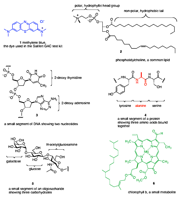
Figure 1. Examples of the molecules of life, and methylene blue, the Salifert GAC test kit reagent.

With this information as background, we can now ask, “What type of dye molecules might resemble, in structure and/or chemical functionality, elements of DOC?” This question, of course, is impossible to answer with precision for the reasons discussed above, but we can make some educated guesses as to what type of chemical units might survive intact, or be formed from, the input species of Figure 1. The fact that DOC is soluble (= dissolved) requires that it contains functional groups which are hydrophilic (= water loving). In addition, the nucleic acids and some of the proteins’ individual amino acid components (e.g., histidine) contain flat 5- and 6-membered nitrogen-containing ring units that are generally resistant to chemical transformation. Therefore, choosing a dye that contains both flat nitrogen-containing rings and water solubilizing charges seems appropriate. This line of reasoning led to the inclusion of Basic Blue 3 (7) in our study, Figure 2. This dye is structurally similar to methylene blue (1) from the Salifert test kit.

The inevitable oxidation and chemical condensations that define much of the pathway from cell metabolite to DOC typically results in the formation of compounds featuring condensed ring systems, and also to the generation of oxidized chemical functionality like carboxylic acids and phenols. One dye that embodies both of these likely DOC characteristics is fluorescein (8), Figure 2. This orange dye might be a simple model for the “humic substances” that contain acids and phenols on rings similar to the presentation depicted in the structure 8.

Many organic molecules of the type produced by biological metabolism have a dual character with respect to water. These molecules have both a hydrophilic portion and a hydrophobic (= water hating) portion, and they are termed amphoteric. Lipids are good examples of amphoteric molecules, as illustrated in Figure 1. In particular, amphoteric molecules might be good candidates for removal by GAC, as the hydrophilic portion will keep them in solution, whereas the hydrophobic portion is similar in character to the binding surface of GAC and therefore is susceptible to strong association. The dye molecule Acid Yellow 76 (9) has just such amphoteric character, as it has both a hydrophilic, charged sulfonate group and a carbon-rich and uncharged tail (Figure 2). In addition, the 6-membered ring residues in 9 are characteristic of many biological metabolites, and this very stable and unreactive ring often survives bacterial action either intact or only slightly modified. Thus, it may serve as a useful model for amphoteric molecules in DOC.

Finally, the common occurrence of porphyrin-based metabolites in cells, and the relative resistance of the porphyrin superstructure to complete degradation (porphyrins are used as biomarkers in geological samples millions of years old (Callot, 2000)), suggests that a dye mimicking this color source might be a useful contributor to modeling DOC in GAC-based removal studies. Towards this end, the porphyrin derivative chlorophyllin (10) was selected as the final probe dye for use in the GAC studies.

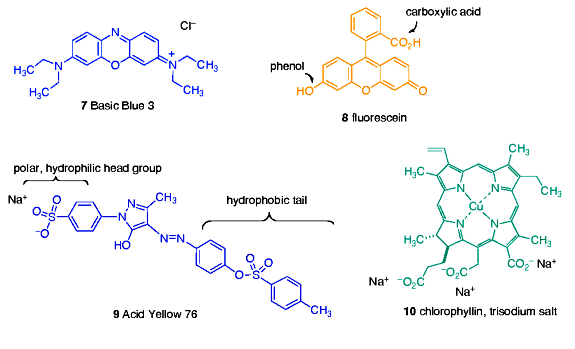
Figure 2. The dyes used in the GAC-based adsorption assays.

These model compounds were chosen for their resemblance to presumed DOC components, although this point cannot be experimentally verified. Argument-by-analogy will be our strongest ally upon employing this modeling approach to investigating GAC’s properties. Thus, using these model compounds will allow us to acquire meaningful data and provide a framework for interpretation of the results, which in turn will, hopefully, provide some guidance for the aquarist contemplating the details of GAC use in his/her aquarium.

In Part 2 next month, we will continue with the Results and Discussion of the data.