

One thing that aquarists have to deal with when designing a new system or reconfiguring an existing system is flow. Part of that overall question is selecting the proper plumbing configuration and selecting a pump for the application.
For the last couple of years there have been online applications that allow an aquarist to enter their plumbing configuration and select a pump to see what kind of flow they would get with their proposed plumbing schematic. A couple drawbacks to the online applications are that they don’t allow you to add new pumps and you can’t save your results after selecting a configuration and running a calculation. Because of the deficiencies (and wanting to delve further into programming), I wrote a program that will allow you to do just that. It is written in the Python programming language and has been open sourced under the GNU General Public License for others to contribute to in hopes of making it better. For those of you who don’t know what open source software is, it’s:
“…computer software whose source code is available under a license (or arrangement such as the public domain) that permits users to study, change, and improve the software, and to redistribute it in modified or unmodified form. It is often developed in a public, collaborative manner. It is the most prominent example of open source development and often compared to user generated content.” (1)
There’s all sorts of open source software available (Sourceforge.net, Google Code, etc) if the reader has never heard of it before.
For those interested in the source code, it can be found on Google Code.
This article will not go over pumps and plumbing design as it was already covered in great detail by Sanjay Joshi, Ph.D. and Nathan Paden in “An Engineering View of Aquarium Systems Design: Pumps and Plumbing.” (2) It will, however, go over installing, using the program, and adding additional pumps to the pumps list.
Download and Installation
Download the program and install it in the normal manner. Currently only a Windows installer is available. If you’re using an alternative operating system like Linux, you will need to install Python 2.4, Tix, and BeautifulSoup before going further. If there is someone out there with Linux expertise that would like to build an installer for Linux (Ubuntu, Fedora Core, etc) email me or submit it on the project site and we can work on it.
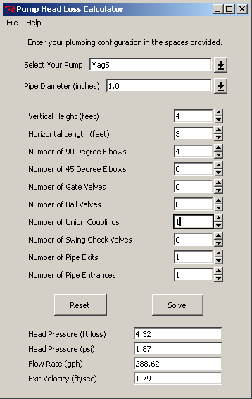
The program entry fields.
Usage
Once you’ve downloaded and installed the software, double click on the icon to start the program. Below is what you’ll see:
To use it, all you have to do is select your pump from the dropdown list, followed by your pipe diameter. Next enter all of your plumbing variables and click the “Solve” button. The results will be printed at the bottom of your screen. You’ll be shown the Head Pressure (ft loss), Head Pressure in pounds/inch (psi), the resulting Flow Rate your system in gallons/hour (gph) and the Exit Velocity of the water coming out of your exit pipe. The program is smart enough that if you tell it that there is more than one Exit in your plumbing diagram, it will divide your water velocity by the number of exits and tell you the exit velocity per plumbing exit. Current limitations of the program are that you cannot select more than one pipe diameter. Multiple pipe diameters make the calculations significantly more complex. The program does assume that you know something about the various pumps when trying to find one for your application. Currently there are over 120 pumps in the database so having a bit of knowledge of the pumps and what they can do beforehand is a plus otherwise you may be selecting a lot of pumps before you find one to your liking.
As mentioned, there are two nice features to this program:
- You can save your results
- You can add your own pumps
Saving your Data
This is pretty straight forward. Go to File – Save and enter the filename you want to save your data as on the filesystem. The program saves your files to a .csv format. .csv is a very simple format that can be read by just about all spreadsheet programs. It can be opened in Excel,
OpenOffice Calc, etc. It makes it very handy when you’re trying to work through multiple plumbing configurations and you want to compare them.
How To Add New Pumps
Adding new pumps to the program is a straight forward process. It can be a bit involved up front as you’ll have to do a bit of leg work to find the pump curve for the pump(s) you want to add to the program. Then it’s a matter of converting that curve into a series of constants that describe it mathmatically. After that it’s as simple as editing a text file.
The steps to add a pump to the program are as follows:
- Obtain a pump curve for the pump you want to add
- Recreate the pump curve in Excel and draw a 3rd degree polynomial through the data set
- Extract the polynomial constants from the equation
- Edit pumps.xml (located in your program folder) and add the constants.
- Restart the program
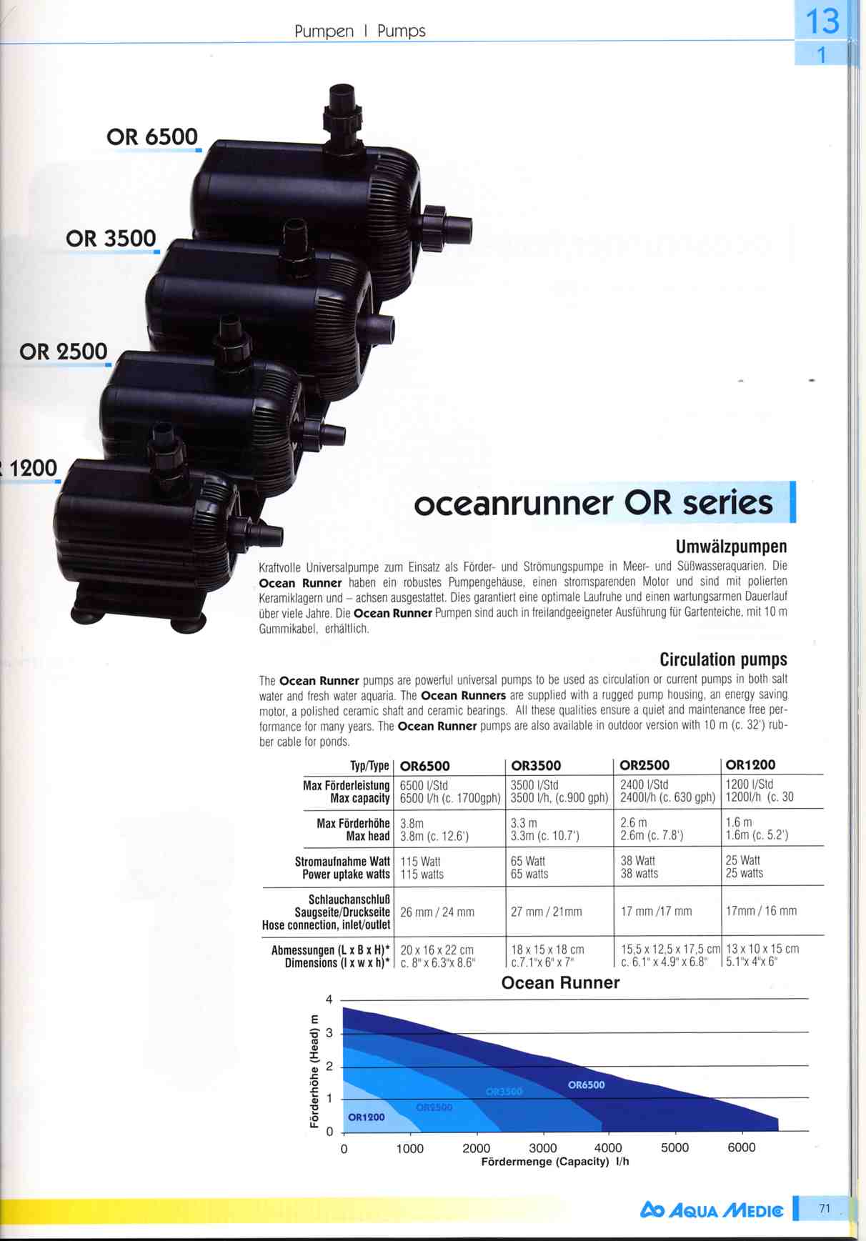
Oceanrunner OR pump specifications.
Obtaining the Pump Curve
The first step is to obtain the pump curve for your pump. Sometimes it’s as simple as doing a Google search for the pump and finding the associated pump curve. Other times you may have to resort to emailing the manufacturer for the pump curve. A lot of it will be digging on your part.
There was a request in a forum post for the Oceanrunner OR series of pumps. The poster included the technical details for the pumps as well as the pump curves for each pump. For this example, I will use the Oceanrunner OR 6500 pump and the technical details for this pump can be found in the following specification:
At the very bottom of this specification sheet is our pump curve. It’s the blue shaded graph that has plots l/h vs. m.
Now that we have the pump curve in our hands, the next step is to recreate the pump curve in Excel or any other spreadsheet that can be used to draw lines through data points.
Recreate the Pump Curve
In this example, I’ll use Microsoft Excel for recreating the pump curve.
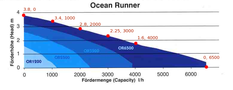
The OR 6500 pump curve with our data points extracted.
Start up your spreadsheet program. The pump curve for the OR 6500 is given in meters vs liters/hour. Basically what we are going to do is extract six data points from the chart and make a table out of it. At six different points on the pump curve, extract the meters and liters/hour values and enter them in your table. The below graph shows our datapoints:
When done you should have a table that looks something like this:
| meters | liters/hour |
|---|---|
| 0 | 6500 |
| 1.6 | 4000 |
| 2.25 | 3000 |
| 2.8 | 2000 |
| 3.4 | 1000 |
| 3.8 | 0 |
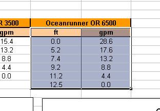
Now we have to do a bit of math. In order to obtain our pump constants, we need our data to be in feet vs. gallons/minute. The following are the conversions from one unit to another:
- 1 meter = 3.28083 feet
- 1 gallon = 0.2641721 liters
- 1 hour = 60 minutes
Using these conversion factors, our table will now look like this:
| feet | gallons/minute |
|---|---|
| 0.0 | 28.6 |
| 5.2 | 17.6 |
| 7.4 | 13.2 |
| 9.2 | 8.8 |
| 11.2 | 4.4 |
| 12.5 | 0.0 |
Selecting our data points.
Now that our data is in the proper format we will graph it to find our pump constants. First, select the region that contains the data points.
Create a graph by either clicking on the Chart Wizard icon in your menu toolbar or by clicking on Insert – Chart menu selections. The Chart Wizard should start up. Select the XY (Scatter) option from the Chart Type selection box and then click the Next > button. Click the Next > button until you get to the place where you can enter a Chart Title, Values (X) axis, and Values (Y) axis. Enter your title as “Oceanrunner OR 6500”, y-axis as “Gallons / Minute”, and your x-axis as “Feet”. With that done, click the Finish button and your chart will be created for you. You’ll now have a chart that looks something like:
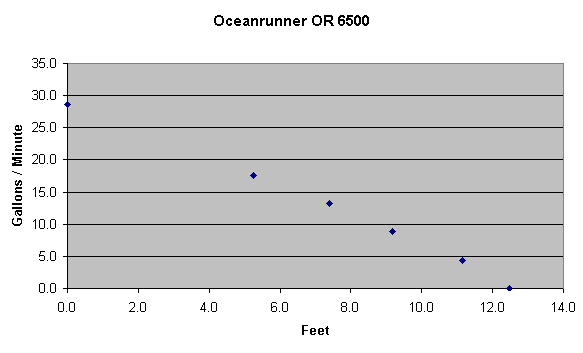
Chart with the proper data now displayed.
Next, we need to plot a line through the data in order to obtain our pump constants. Click on one of the dots on the chart that was just drawn and then right click and select “Add Trendline” from the menu. In the Type tab, select “Polynomial” and increase the “Order” from 2 to 3 in the box beside it. Now click on the Options tab of that window and check the “Display equation on chart” and click OK. A 3rd degree polynomial is now displayed on your chart. Right click on the equation and select “Format Data Labels.” On that window, select the Number tag and in the Category box, select Number and increase the Decimal Places from ‘2’ to ’10’ and click OK when done. Now we have a line equation that describes our pump curve. From this we can easily pull out our pump constants.
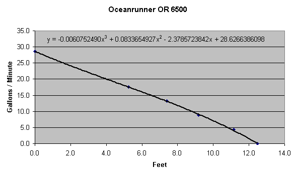
The resulting graph with the line equation on it.
The line equation should loook something like:
y = ax^3 + bx^2 + cx + d
From this equation we can easily extract our pump constants.
Now we will actually add our pump to the list of pumps that is selectable in our program. Open up Windows Explorer and navigate to where you installed your Calculator (default is C:Program FilesPump Head Loss Calculator) and open pumps.xml in a text editor like Notepad. Scanning through the file you’ll see a lot of:
<pump name="Mag24">
<a>-0.004946242991993064</a>
<b>0.1253160569978384</b>
<c>-2.761630952530459</c>
<d>40.04301814394783</d>
</pump>
What we are going to do is copy a section and add our pump name and pump constants to the appropriate places.
If you look over the code in the file you’ll see it’s pretty straight forward. Every pump is defined within a <pump /> tag in an attributed named (obviously) “name”. Our pump constants can be found nested inside this tag in <a />, <b />, <c />, or <d /> tags.
A short <info /> tag is placed at the very beginning of the pumps.xml file in order to remind anyone adding pumps to the list exactly how it should be done. It’s there as a matter of convenience so that you don’t have to refer back to this article to remember how to do it.
Copy a <pump /> section and paste it right below the last pump in the list. Now, edit the “name” attribute by replacing the text within the quotation marks with “Oceanrunner OR 6500”. Now, edit each of the <a />, <b />, <c />, and <d /> tags and place the appropriate constants within each tag. “a” represents the constant in from of x^3, b represents the constant in from of x^2, c represents the constant in from of x, and d represents the constant at the very end of our equation. If there is a negative sign in front of a constant, make certain to add that in as well. Make certain that you have no extra spaces within your <a />, <b />, <c />, or <d /> tags as this might throw an error in our program.
Below is what your addition should look like:
<pump name="Oceanrunner OR 6500">
<a>-0.0060752490</a>
<b>0.0833654927</b>
<c>-2.3785723842</c>
<d>28.6266386098</d>
</pump>
Once that is done, save the file and re-run the Pump Head Loss Calculator. With any luck your pump will now be added to the list.
Conclusions
I hope that you enjoy the program. If you happen to add new pumps to the program, by all means contribute those pumps on the project page at Google Code. Please submit bug reports, code fixes, suggestions, etc to the project as the users will make this a better program overall.
Enjoy!
References
- Open-source software, Wikipedia, http://en.wikipedia.org/wiki/Open_source_software
- An Engineering View of Aquarium Systems Design: Pumps and Plumbing by Sanjay Joshi, Ph.D., Nathan Paden, and Shane Graber, Volume 2, Issue 1, Advanced Aquarist’s Online Magaine (http://www.advancedaquarist.com/issues/jan2003/featurejp.htm)

0 Comments